![]()
![]()
This R package provides helper functions I found useful when developing R code - perhaps you will too! The released package version can be installed via:
install.packages("oeli")The following shows some demos. Click the headings for references on all available helpers in each category.
The hermann data contains historical information on
editions of the Hermannslauf,
including the date, temperature, and winning times for men and
women:
hermann
#> # A tibble: 54 × 8
#>    edition  year date        temp winner_men        seconds_men winner_women
#>      <dbl> <dbl> <date>     <dbl> <chr>                   <dbl> <chr>
#>  1       1  1972 1972-04-16    NA Helmut Bode              6686 Lydia Günnewig
#>  2       2  1973 1973-04-29    14 Helmut Bode              6795 Irmhild Holste
#>  3       3  1974 1974-04-28    14 Achim Stober             6942 Liane Winter
#>  4       4  1975 1975-04-27    11 Klaus-Dieter Holz        6720 Christine Ross
#>  5       5  1976 1976-04-25    11 Heribert Bulk            6453 Liane Winter
#>  6       6  1977 1977-04-24     9 Jim Hodey                6503 Liane Winter
#>  7       7  1978 1978-04-30    16 Michael Heine            6856 Liane Winter
#>  8       8  1979 1979-04-29     7 Billy Cain               6587 Liane Winter
#>  9       9  1980 1980-04-27     9 Dieter Lippe             6706 Liane Winter
#> 10      10  1981 1981-04-26    16 Helmut Schmidt           6735 Rotraud Zinner
#> # ℹ 44 more rows
#> # ℹ 1 more variable: seconds_women <dbl>The package has density and sampling functions for some distributions not included in base R, like the Dirichlet:
ddirichlet(x = c(0.2, 0.3, 0.5), concentration = 1:3)
#> [1] 4.5
rdirichlet(concentration = 1:3)
#> [1] 0.01795087 0.41315984 0.56888929
Or the mixture of Gaussian distributions:
x <- c(0, 0)
mean <- matrix(c(1, 1, -1, -1), ncol = 2) # means in columns
Sigma <- matrix(c(diag(2), 0.1 * diag(2)), ncol = 2) # vectorized covariances in columns
proportions <- c(0.7, 0.3)
dmixnorm(x = x, mean = mean, Sigma = Sigma, proportions = proportions)
#> [1] 0.04100656
pmixnorm(x = x, mean = mean, Sigma = Sigma, proportions = proportions)
#> [1] 0.3171506
rmixnorm(n = 1000, mean = mean, Sigma = Sigma, proportions = proportions) |>
  as.data.frame() |>
  ggplot2::ggplot() + ggplot2::geom_point(ggplot2::aes(x = V1, y = V2))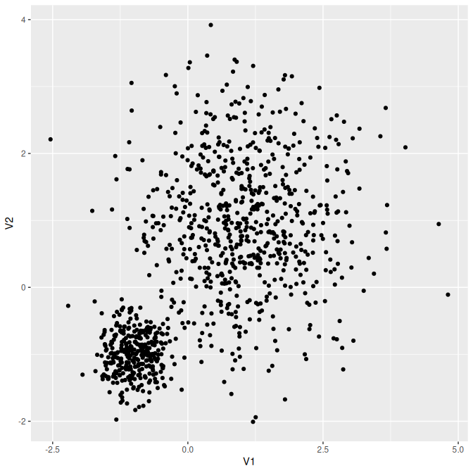
Retrieving default arguments of a function:
f <- function(a, b = 1, c = "", ...) { }
function_defaults(f)
#> $b
#> [1] 1
#>
#> $c
#> [1] ""Create all possible permutations of vector elements:
permutations(LETTERS[1:3])
#> [[1]]
#> [1] "A" "B" "C"
#>
#> [[2]]
#> [1] "A" "C" "B"
#>
#> [[3]]
#> [1] "B" "A" "C"
#>
#> [[4]]
#> [1] "B" "C" "A"
#>
#> [[5]]
#> [1] "C" "A" "B"
#>
#> [[6]]
#> [1] "C" "B" "A"Quickly have a basic logo for your new package:
logo <- package_logo("my_package", brackets = TRUE)
print(logo)![]()
How to print a matrix without filling up the entire
console?
x <- matrix(rnorm(10000), ncol = 100, nrow = 100)
print_matrix(x, rowdots = 4, coldots = 4, digits = 2, label = "what a big matrix")
#> what a big matrix : 100 x 100 matrix of doubles
#>         [,1]  [,2] [,3] ... [,100]
#> [1,]    -0.3 -0.74 -0.1 ...   1.01
#> [2,]    1.39 -2.06 1.29 ...   -0.5
#> [3,]   -0.45 -1.57 0.43 ...   1.61
#> ...      ...   ...  ... ...    ...
#> [100,]  1.12  0.77 -1.6 ...  -0.08
And what about a data.frame?
x <- data.frame(x = rnorm(1000), y = LETTERS[1:10])
print_data.frame(x, rows = 7, digits = 0)
#>      x  y
#> 1     0 A
#> 2     1 B
#> 3     0 C
#> 4    -1 D
#> <993 rows hidden>
#>
#> 998   0 H
#> 999   0 I
#> 1000 2 JLet’s simulate correlated regressor values from different marginal distributions:
labels <- c("P", "C", "N1", "N2", "U")
n <- 100
marginals <- list(
  "P" = list(type = "poisson", lambda = 2),
  "C" = list(type = "categorical", p = c(0.3, 0.2, 0.5)),
  "N1" = list(type = "normal", mean = -1, sd = 2),
  "U" = list(type = "uniform", min = -2, max = -1)
)
correlation <- matrix(
  c(1, -0.3, -0.1, 0, 0.5,
    -0.3, 1, 0.3, -0.5, -0.7,
    -0.1, 0.3, 1, -0.3, -0.3,
    0, -0.5, -0.3, 1, 0.1,
    0.5, -0.7, -0.3, 0.1, 1),
  nrow = 5, ncol = 5
)
data <- correlated_regressors(
  labels = labels, n = n, marginals = marginals, correlation = correlation
)
head(data)
#>   P C        N1         N2         U
#> 1 3 3  0.854606 -1.1509971 -1.575507
#> 2 3 3 -3.801998  0.5696389 -1.784321
#> 3 4 3 -1.024611 -1.0414976 -1.333803
#> 4 0 3 -0.490758 -0.9806894 -1.840349
#> 5 1 3 -1.681134  0.7511786 -1.939042
#> 6 2 1 -2.814986  0.7984411 -1.367265
cor(data)
#>              P          C          N1          N2          U
#> P   1.00000000 -0.2287181 -0.08793083 -0.02476611  0.4877251
#> C  -0.22871807  1.0000000  0.28573358 -0.52539377 -0.7628656
#> N1 -0.08793083  0.2857336  1.00000000 -0.30000000 -0.2694518
#> N2 -0.02476611 -0.5253938 -0.30000000  1.00000000  0.1138354
#> U 0.48772506 -0.7628656 -0.26945184 0.11383544 1.0000000The group_data.frame() function groups a given
data.frame based on the values in a specified column:
df <- data.frame("label" = c("A", "B"), "number" = 1:10)
group_data.frame(df = df, by = "label")
#> $A
#>   label number
#> 1     A      1
#> 3     A      3
#> 5     A      5
#> 7     A      7
#> 9     A      9
#>
#> $B
#>    label number
#> 2      B      2
#> 4      B      4
#> 6      B      6
#> 8      B      8
#> 10 B 10Is my matrix a proper transition probability matrix?
matrix <- diag(4)
matrix[1, 2] <- 1
check_transition_probability_matrix(matrix)
#> [1] "Must have row sums equal to 1"