The main content of pedprobr is an implementation of the Elston-Stewart algorithm for pedigree likelihoods given marker genotypes. It is part of the pedsuite, a collection of packages for pedigree analysis in R.
The pedprobr package does much of the hard work in several other pedsuite packages:
The workhorse of pedprobr is the
likelihood() function, which supports a variety of
situations:
To get the current official version of pedprobr, install from CRAN as follows:
install.packages("pedprobr")Alternatively, get the latest development version from GitHub:
# install.packages("devtools") # install devtools if needed
devtools::install_github("magnusdv/pedprobr")library(pedprobr)
#> Loading required package: pedtoolsTo set up a simple example, we first use pedtools
utilities to create a pedigree where two brothers are genotyped with a
single SNP marker. The marker has alleles a and
b, with frequencies 0.2 and 0.8 respectively, and both
brothers are heterozygous a/b.
# Pedigree with SNP marker
x = nuclearPed(nch = 2) |>
  addMarker(geno = c(NA, NA, "a/b", "a/b"), afreq = c(a = 0.2, b = 0.8), name = "M1")

# Plot with genotypes
plot(x, marker = "M1")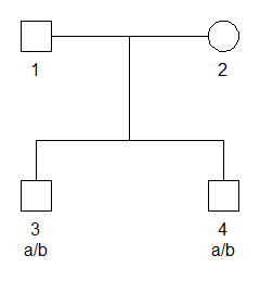
The pedigree likelihood, i.e., the probability of the genotypes given the pedigree, is obtained as follows:
likelihood(x)
#> [1] 0.1856Besides likelihood(), other important functions in
pedprobr are:
oneMarkerDistribution(): the joint genotype
distribution at a single marker, for any subset of pedigree memberstwoMarkerDistribution(): the joint genotype
distribution at two linked markers, for a single personIn both cases, the distributions are computed conditionally on any known genotypes at the markers in question.
To illustrate oneMarkerDistribution() we continue our
example from above, and consider the following question: What is
the joint genotype distribution of the parents, conditional on the
genotypes of the children?
The answer is found as follows:
oneMarkerDistribution(x, ids = 1:2, verbose = F)
#>            a/a        a/b       b/b
#> a/a 0.00000000 0.01724138 0.1379310
#> a/b 0.01724138 0.13793103 0.2758621
#> b/b 0.13793103 0.27586207 0.0000000
The output confirms the intuitive result that the parents cannot both
be homozygous for the same allele. The most likely combination is that
one parent is heterozygous a/b, while the other is
homozygous b/b.
The argument output controls how the output of
oneMarkerDistribution() is formatted. Instead of the
default matrix (or multidimensional array, if more than 2 individuals),
we can also get the distribution in table format:
oneMarkerDistribution(x, ids = 1:2, verbose = F, output = "table")
#>     1   2       prob
#> 1 a/a a/a 0.00000000
#> 2 a/b a/a 0.01724138
#> 3 b/b a/a 0.13793103
#> 4 a/a a/b 0.01724138
#> 5 a/b a/b 0.13793103
#> 6 b/b a/b 0.27586207
#> 7 a/a b/b 0.13793103
#> 8 a/b b/b 0.27586207
#> 9 b/b b/b 0.00000000
A third possibility is output = "sparse", which gives a
table similar to the above, but with only the rows with non-zero
probability.