jamba
The goal of jamba is to provide useful custom functions for R data
analysis and visualization. jamba version 1.0.2
Package Reference
A full online function reference is available via the pkgdown
documentation:
Full jamba command
reference
Functions are categorized, some examples are listed below:
Installation
Production will soon be available from CRAN:
install.packages("jamba")
The development version can be installed:
remotes::install_github("jmw86069/jamba")
Additional R Packages in
“Suggests”
crayon - install with
install.packages("crayon") for glorious colored console
output. Color makes it better.farver - install with
install.packages("farver") for more efficient color
manipulations, and HSL color coneversions.
Additional R Packages in
“Enhances”
Bioconductor packages are invaluable for bioinformatics work, but can
be a bit “heavy” to install if not absolutely necessary. Therefore,
Bioconductor packages are in “Enhances” so they require someone to make
the choice to install them.
S4Vectors - install with
BiocManager::install("S4vectors") to improve speed of
cPaste() functions.openxlsx - install with
install.packages("openxlsx") to support Excel
xlsx file import, and stylized export.kableExtra - install with
install.packages("kableExtra") to enable colorized kable
HTML tables in RMarkdown documents.ComplexHeatmap - install with
BiocManager::install("ComplexHeatmap") to use with
heatmap_row_order(), cell_fun_label() for
custom labels.matrixStats - install with
install.packages("matrixStats") for efficient
numeric stats calculations, or
sparseMatrixStats for use with Matrix sparse matrices as
used with Seurat and SingleCellExperiment data.ggridges - install with
install.packages("ggridges") for convenient ridge density
plots using plotRidges().
Background
The R functions in jamba have been built up, used,
tested, revised over several years. They are immediately useful for
day-to-day work, and efficient and robust enough for production
pipelines.
Many were inspired by discussion from Stackoverflow, R-help, or
Bioconductor, with citations thanking principal author(s). Many thanks
to the original authors! The R community is built upon the collective
greatness of its contributors!
Most of the functions are designed around workflows for
Bioinformatics analyses, where functions need to be efficient when
operating over 10,000 to 100,000 elements. (They work quite well with
millions as well.) Usually the speed gains are obvious with about 100
elements, then scale linearly (or worse) as the number increases. I and
others use these functions all the time.
One example function writeOpenxlsx() is a simple wrapper
around very useful openxlsx::write.xlsx(), which also
applies column formatting for column types: P-values, fold changes, log2
fold changes, numeric, and integer values. Columns use conditional Excel
formatting to apply color-shading to cells for each type.
Similarly, readOpenxlsx() is a wrapper function to
openxlsx::read.xlsx() which reads each worksheet and
returns a list of data.frame objects. It can
detect multi-row column headers, for which it returns combined column
names. It also applies equivalent of check.names=FALSE so
column names are returned without change.
Small and large efficiencies are used wherever possible. The
mixedSort() functions are based upon
gtools::mixedsort(), with additional optimizations for
speed and custom needs. It sorts chromosome names, gene names, micro-RNA
names, etc.
Alphanumeric sort
mixedSort() - highly efficient alphanumeric sort, for
example chr1, chr2, chr3, chr10, etc.mixedSortDF() - as above, applied to columns in a
data.frame (or matrix, tibble,
DataFrame, etc.)mixedSorts() - as above, applied to a list of vectors
with no speed loss.
Example:
| 2 |
ABCA2 |
2 |
1 |
| 1 |
ABCA12 |
1 |
2 |
| 3 |
miR-1 |
3 |
3 |
| 6 |
miR-1a |
6 |
4 |
| 7 |
miR-1b |
7 |
5 |
| 8 |
miR-2 |
8 |
6 |
| 4 |
miR-12 |
4 |
7 |
| 9 |
miR-22 |
9 |
8 |
| 5 |
miR-122 |
5 |
9 |
Base R plotting
These functions help with base R plots, in all those little cases
when the amazing ggplot2 package is not a smooth fit.
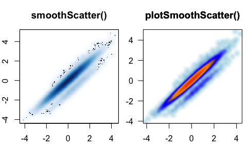
nullPlot() - convenient “blank” base R plot, optionally
displays marginsplotSmoothScatter() - smooth scatter
plot() for point density, enhanced over
smoothScatter()
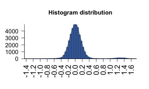
plotPolygonDensity() - fast density/histogram plot for
vector or matrix
imageDefault() - enhanced image() that
enables raster output with consistent pixel aspect ratio.imageByColors() - wrapper to image() for a
matrix or data.frame of colors, with optional labels
minorLogTicksAxis(), logFoldAxis(),
pvalueAxis() - log axis tick marks and labels, compatible
with offset for example log(offset + x).sqrtAxis() - draw a square-root transformed axis, with
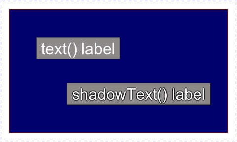
proper labels.drawLabels() - draw square colorized text labelsshadowText() - replacement for text() that
draws shadows or outlines.
groupedAxis() - grouped axis labels to show
regions/rangesdecideMfrow() - determine appropriate value for
par("mfrow") for multipanel output in base R plotting.getPlotAspect() - determine visible plot aspect
ratio.
Excel export
Every Bioinformatician/statistician needs to write data to Excel, the
writeOpenxlsx() function is consistent and makes it look
pretty. You can save numerous worksheets in a single Excel file, without
having to go back and custom-format everything.
writeOpenxlsx() - flexible Excel exporter, with
categorical and conditional colors.applyXlsxCategoricalFormat() - apply categorical colors
to ExcelapplyXlsxConditionalFormat() - apply conditional colors
to Excel
Colors
Almost everything uses color somewhere, especially on R console, and
in every R plot.
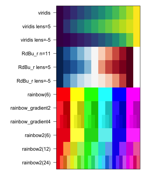
getColorRamp() - retrieve or create color palettessetTextContrastColor() - find contrasting font color
for colored backgroundmakeColorDarker() - make a color darker (or lighter, or
saturated)color2gradient() - split one color to a gradient of
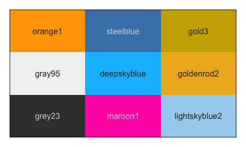
n colorsshowColors() - display a vector or list of
colorsrainbow2() - enhances rainbow()
categorical colors for visual contrast.warpRamp() - “bend” a color gradient to enhance the
visual rangefixYellow() - opinionated reduction of yellow-green
hueprintDebug() - colorized text output to console or
RMarkdownprintDebugHtml() - colorized HTML output in RMarkdown
or web pageskable_coloring() - colored
kableExtra::kable() RMarkdown tables, if
kableExtra package is installed.col2alpha(), alpha2col() - get or set
alpha transparencycol2hcl(), col2hsl(),
col2hsv(), hcl2col(), hsl2col(),
hsv2col(), rgb2col() - consistent color
conversions.color_dither() - split color into two to make color
stripes
List Functions
Efficient methods to operate on lists in one call, to avoid looping
through the list either with for() loops,
lapply() or map() functions. Driven by speed
with 10k-100k rows, typical biological datasets.
Compared to convenient alternatives, apply() or
tidyverse, typically order of magnitude faster. (Ymmv.) Notable
exceptions: data.table and Bioconductor
S4Vectors. Both are amazing, and are fairly heavy
installations. S4Vectors is used when available.
cPaste() - paste(..., collapse) a list of
vectorscPasteS() - cPaste() with
mixedSort()cPasteU() - cPaste() with
unique() (actually uniques())cPasteSU() - cPaste() with
mixedSort() and unique()uniques() - unique() across a list of
vectorssclass() - class() a listsdim() - dim() across a list, or S4
object, or non-list objectssdim() - sdim() across a listsdima() - sdim() for
attributes()rbindList() - do.call(rbind, ...) to bind
rows into a matrix or data.frame, useful
together with strsplit().mergeAllXY() -
merge(..., all.x=TRUE, all.y=TRUE) a list of
data.framermNULL() - remove NULL from a list, with optional
replacementrmNAs() - rmNA() across a list, with
option replacement(s)showColors() - display colorsheads() - head() across a list
Unique names with versions
R object names provide an additional method to confirm data are kept
in the proper order. Duplicated names may be silently ignored, which
motivated the easy approach to “make unique names”.
makeNames() - make unique names, with flexible
rulesnameVector() - add unique names using
makeNames()nameVectorN() - make vector of names, named with
makeNames(). Useful inside lapply() which
returns names but only when provided.
data.frame/matrix/tibble
mixedSortDF() - mixedSort() by columns or
rownamespasteByRow() - fast row-paste with delimiters, default
skips blankspasteByRowOrdered() - nifty alternative that honors
factor levelsrowGroupMeans(), rowRmMadOutliers() -
grouped row functionsmergeAllXY() - merge a list of data.frame
into one, keeping all rowsrenameColumn() - rename columns from and
to.kable_coloring() - flexible colorized
data.frame output in Rmarkdown.
String / grep
tcount() - table() sorted high-to-low,
with minimum count filtermiddle() - show n entries from start,
middle, then end.gsubOrdered() - gsub() that returns
ordered factor, inherits existinggsubs() - gsub() a vector of
patterns/replacements.grepls() - grep the environment object names, including
attached packagesvgrep(), vigrep() - value-grep
shortcutunvgrep(), unvigrep() - un-grep, remove
matched resultsprovigrep() - progressive grep, returns matches in
order of patternsigrepHas() - case-insensitive grep-anyucfirst() - upper-case the first letter of each
word.padString(), padInteger() - produce
strings from numeric values with consistent leading zeros.
Numeric
formatInt() - opinionated format() for
integers.normScale() - scale between 0 and 1 or custom
rangenoiseFloor() - apply noise floor, ceiling, with
flexible replacementslog2signed(), exp2signed() - log2 with
offset, and reciprocalrowGroupMeans(), rowRmMadOutliers() -
efficient grouped row functionsdeg2rad(), rad2deg() - interconvert
degrees and radiansrmNA() - remove NA values, with optional
replacementwarpAroundZero() - warp a numeric vector symmetrically
around zerormInfinite() - remove infinite values, with optional
replacement.formatInt() - convenient format() for
integer output, with comma-delimiter by default
Common usage
noiseFloor(0:10, minimum=1e-20, newValue=NA)
#>  [1] NA  1  2  3  4  5  6  7  8  9 10
- convert values below floor to floor:
noiseFloor(0:10, minimum=3)
#>  [1]  3  3  3  3  4  5  6  7  8  9 10
- convert values below floor or NA to floor:
noiseFloor(c(0:10, NA), minimum=3, adjustNA=TRUE)
#>  [1]  3  3  3  3  4  5  6  7  8  9 10  3
Practical / helpful
jargs() - pretty function arguments, optional pattern
search argument name
jargs(plotSmoothScatter)
#>                 x = ,
#>                 y = NULL,
#>              bwpi = 50,
#>             binpi = 50,
#>        bandwidthN = NULL,
#>              nbin = NULL,
#>            expand = c(0.04, 0.04),
#>       transFactor = 0.25,
#>    transformation = function( x ) x^transFactor,
#>              xlim = NULL,
#>              ylim = NULL,
#>              xlab = NULL,
#>              ylab = NULL,
#>          nrpoints = 0,
#>           colramp = c("white", "lightblue", "blue", "orange", "orangered2"),
#>               col = "black",
#>            doTest = FALSE,
#>    fillBackground = TRUE,
#>          naAction = c("remove", "floor0", "floor1"),
#>              xaxt = "s",
#>              yaxt = "s",
#>               add = FALSE,
#>               asp = NULL,
#> applyRangeCeiling = TRUE,
#>         useRaster = TRUE,
#>           verbose = FALSE,
#>               ... =
sdim(), ssdim() - dimensions of list
objects, or nested list of listssdima() - runs sdim() on the attributes of
an object.isTRUEV(), isFALSEV() - vectorized test
for TRUE or FALSE values, since isTRUE() only operates on
single values, and does not allow NA.reload_rmarkdown_cache() - load RMarkdown cache folder
into environmentcall_fn_ellipsis() - for developers, call child
function while passing only acceptable arguments in ....
Instead of: something(x, ...), use:
call_fn_ellipsis(something, x, ...) and never worry about
....log2signed(), exp2signed() - convenient
log2(1 + x) or its reciprocal, using customizable
offset.newestFile() - most recently modified file from a
vector of files
R console
jargs() - Jam argument list - see “Practical” above for
examplelldf() - ls() with
object.size() into data.framemiddle() - Similar to head() and
tail(), middle() shows n entries
from beginning, middle, to end.printDebug() - colorized text outputsetPrompt() - colorized R console prompt with project
name and R version
RMarkdown
reload_rmarkdown_cache() - when rendering RMarkdown
with cache=TRUE, this function reads the cache to reload
the environment without re-processing, to recover the exact result for
continued work.
printDebugHtml() - colored HTML output.
- Shortcut for
printDebug(..., htmlOut=TRUE, comments=FALSE), or
options("jam.htmlOut"=TRUE, "jam.comment"=FALSE).
- The RMarkdown chunk must include:
results='asis'
printDebugHtml("printDebugHtml(): ",
  "Output is colorized: ",
  head(LETTERS, 8))
(12:05:41) 07Mar2025: printDebugHtml(): Output is colorized: A,B,C,D,E,F,G,H
withr::with_options(list(jam.htmlOut=TRUE, jam.comment=FALSE), {
  printDebugHtml(c("printDebug() using withr::with_options(): "),
    c("Output should be colorized: "),
    head(LETTERS, 8));
})
(12:05:41) 07Mar2025: printDebug() using withr::with_options():
Output should be colorized:
A,B,C,D,E,F,G,H
expt_df <- data.frame(
  Sample_ID="",
  Treatment=rep(c("Vehicle", "Dex"), each=6),
  Genotype=rep(c("Wildtype", "Knockout"), each=3),
  Rep=paste0("rep", c(1:3)))
expt_df$Sample_ID <- pasteByRow(expt_df[, 2:4])

# define colors
colorSub <- c(Vehicle="palegoldenrod",
  Dex="navy",
  Wildtype="gold",
  Knockout="firebrick",
  nameVector(color2gradient("grey48", n=3, dex=10), rep("rep", 3), suffix=""),
  nameVector(
    color2gradient(n=3,
      c("goldenrod1", "indianred3", "royalblue3", "darkorchid4")),
    expt_df$Sample_ID))
kbl <- kable_coloring(
  expt_df,
  caption="Experiment design table showing categorical color assignment.",
  colorSub)
Jam Github R packages are being transitioned to
CRAN/Bioconductor:
venndir: Venn diagrams with direction, designed for
published figures.multienrichjam: Multi-enrichment pathway analysis and
visualization tools.splicejam: Sashimi plots for RNA-seq coverage and
junction data.jamma: MA-plots as a unified data
signal quality control toolset.colorjam: rainbowJam(), Categorical colors
with improved visual contrast.genejam: Fast, structured approach to gene symbol
integration.platjam: Platform specific functions: Nanostring,
Salmon, Proteomics, Lipidomics; NGS coverage heatmaps.jamses: heatmap_se() friendly wrapper for
ComplexHeatmap; other integrated methods for factor-aware
design/contrasts, normalization, contrasts, heatmaps.jamsession: properly save/load R objects, R sessions, R
functions.