![]()
![]()
This package provides a set of functions to make working with date and datetime data much easier!
While most time-based packages are designed to work with clean and pre-aggregate data, timeplyr contains a set of tidy tools to complete, expand and summarise both raw and aggregate date/datetime data.
Significant efforts have been made to ensure that grouped calculations are fast and efficient thanks to the excellent functionality within the collapse package.
You can install and load timeplyr using the below
code.
# CRAN version
install.packages("timeplyr")

# Development version
remotes::install_github("NicChr/timeplyr")library(timeplyr)
library(tidyverse)
#> ── Attaching core tidyverse packages ──────────────────────── tidyverse 2.0.0 ──
#> ✔ dplyr 1.1.4 ✔ readr 2.1.5
#> ✔ forcats 1.0.0 ✔ stringr 1.5.1
#> ✔ ggplot2 3.5.1 ✔ tibble 3.2.1
#> ✔ lubridate 1.9.4 ✔ tidyr 1.3.1
#> ✔ purrr 1.0.4
#> ── Conflicts ────────────────────────────────────────── tidyverse_conflicts() ──
#> ✖ dplyr::filter() masks stats::filter()
#> ✖ dplyr::lag() masks stats::lag()
#> ✖ ggplot2::resolution() masks timeplyr::resolution()
#> ℹ Use the conflicted package (<http://conflicted.r-lib.org/>) to force all conflicts to become errors
library(fastplyr)
#>
#> Attaching package: 'fastplyr'
#>
#> The following object is masked from 'package:dplyr':
#>
#> desc
#>
#> The following objects are masked from 'package:tidyr':
#>
#> crossing, nesting
library(nycflights13)
library(lubridate)start <- dmy("01-01-2000")
start |>
time_add("year")
#> [1] "2001-01-01"Internally timeplyr makes use of custom timespan objects
for various time manipulations.
timespan("months"); timespan("1 month"); timespan(months(1))
#> <Timespan:months>
#> [1] 1
#> <Timespan:months>
#> [1] 1
#> <Timespan:months>
#> [1] 1

timespan("weeks", 1:10)
#> <Timespan:weeks>
#>  [1]  1  2  3  4  5  6  7  8  9 10
# Parsing
start |> time_add("10 years"); start |> time_add("decade")
#> [1] "2010-01-01"
#> [1] "2010-01-01"

# Lubridate style timespans

start |>
  time_add(years(1))
#> [1] "2001-01-01"

start |> time_add(dyears(1)); start |> time_add("31557600 seconds")
#> [1] "2000-12-31 06:00:00 UTC"
#> [1] "2000-12-31 06:00:00 UTC"

# timeplyr timespans

start |>
  time_add(timespan("years", 1))
#> [1] "2001-01-01"
start |>
  time_add(timespan("years", 0:10))
#>  [1] "2000-01-01" "2001-01-01" "2002-01-01" "2003-01-01" "2004-01-01"
#>  [6] "2005-01-01" "2006-01-01" "2007-01-01" "2008-01-01" "2009-01-01"
#> [11] "2010-01-01"
Time arithmetic involving days, weeks, months and years is equivalent to using lubridate periods.
Any arithmetic involving units less than days, e.g. hours, minutes and seconds, uses normal duration arithmetic in terms of how many seconds have passed. This is equivalent to using lubridate durations.
# Clocks go back 1 hour at exactly 2 am
dst <- dmy_hms("26-10-2025 00:00:00", tz = "GB") |> time_add("hour")

# Below 2 are equivalent
dst |>
  time_add(timespan("hours", 0:2))
#> [1] "2025-10-26 01:00:00 BST" "2025-10-26 01:00:00 GMT"
#> [3] "2025-10-26 02:00:00 GMT"
dst + dhours(0:2)
#> [1] "2025-10-26 01:00:00 BST" "2025-10-26 01:00:00 GMT"
#> [3] "2025-10-26 02:00:00 GMT"

# There is currently no timeplyr way to achieve the below result
# 1 hour forward in clock time is actually 2 literal hours forward
dst + hours(0:2)
#> [1] "2025-10-26 01:00:00 BST" "2025-10-26 02:00:00 GMT"
#> [3] "2025-10-26 03:00:00 GMT"
Period-based hours, minutes and seconds are not as commonly used as literal duration-based hours, minutes and seconds. Therefore timeplyr tries to simplify things by removing the distinction and automatically choosing periods for units larger than an hour and durations for units smaller than a day without the user having to contemplate which to use.
# The lubridate and timeplyr equivalents

time_add(dst, "second"); dst + dseconds(1)
#> [1] "2025-10-26 01:00:01 BST"
#> [1] "2025-10-26 01:00:01 BST"
time_add(dst, "minute"); dst + dminutes(1)
#> [1] "2025-10-26 01:01:00 BST"
#> [1] "2025-10-26 01:01:00 BST"
time_add(dst, "hour"); dst + dhours(1)
#> [1] "2025-10-26 01:00:00 GMT"
#> [1] "2025-10-26 01:00:00 GMT"
time_add(dst, "day"); dst + days(1)
#> [1] "2025-10-27 01:00:00 GMT"
#> [1] "2025-10-27 01:00:00 GMT"
time_add(dst, "week"); dst + weeks(1)
#> [1] "2025-11-02 01:00:00 GMT"
#> [1] "2025-11-02 01:00:00 GMT"
time_add(dst, "month"); dst + months(1)
#> [1] "2025-11-26 01:00:00 GMT"
#> [1] "2025-11-26 01:00:00 GMT"
time_add(dst, "year"); dst + years(1)
#> [1] "2026-10-26 01:00:00 GMT"
#> [1] "2026-10-26 01:00:00 GMT"
Time differences are accurate and simple
start <- today()
end <- today() |>  time_add("decade")

time_diff(start, end, "years")
#> [1] 10

for (unit in .period_units){
    cat(unit, ":", time_diff(start, end, unit), "\n")
}
#> seconds : 315532800
#> minutes : 5258880
#> hours : 87648
#> days : 3652
#> weeks : 521.7143
#> months : 120
#> years : 10When months and years are involved, timeplyr rolls impossible dates forward by default which is different to lubridate which rolls backwards by default
leap <- dmy("29-02-2020")

leap |> time_add("year"); leap |> add_with_rollback(years(1))
#> [1] "2021-03-01"
#> [1] "2021-02-28"
timeplyr handles month addition symmetrically by rolling backwards when adding negative months
leap |> time_subtract("year")
#> [1] "2019-02-28"
This can all be controlled through the roll_month
argument which has options ‘xfirst’, ‘xlast’, ‘preday’, ‘postday’,
‘boundary’, ‘full’ and ‘NA’. The ‘xfirst’ and ‘xlast’ options are
timeplyr specific and signify crossed-first and crossed-last dates
respectively. ‘xlast’ is set by default package-wide.
The choice of rolling impossible dates can affect time difference calculations.
# timeplyr
leap_almost_one_year_old <- dmy("28-02-2021")
cat("timeplyr: ", time_diff(leap, leap_almost_one_year_old, "years"), "\n",
    "lubridate: ", interval(leap, leap_almost_one_year_old) / years(1),
    sep = "")
#> timeplyr: 0.9972678
#> lubridate: 1
In the above example timeplyr lets leaplings be younger for an extra day!
Monthly time differences in timeplyr are symmetric, regardless if
x > y or x < y
time_diff(leap, dmy("28-02-2021") + days(0:1), "years")
#> [1] 0.9972678 1.0000000
time_diff(leap, dmy("01-03-2019") - days(0:1), "years")
#> [1] -0.9972678 -1.0000000

# Not symmetric
interval(leap, dmy("28-02-2021") + days(0:1)) / years(1)
#> [1] 1.00000 1.00274
interval(leap, dmy("01-03-2019") - days(0:1)) / years(1)
#> [1] -0.9972678 -1.0000000timeplyr makes use of its own custom time intervals. These are
intervals of a fixed width. For example, R Dates can be thought of as
fixed intervals of exactly 1 day width. In fact if you call
time_interval() on a Date vector this is exactly what you
get.
time_interval(today())
#> <time_interval> [width:1D]
#> [1] [2025-02-28, +1D)
Going into more detail, timeplyr uses the ‘resolution’ of the object to calculate the default width. Here, ‘resolution’ is defined as the ‘smallest timespan that differentiates two non-fractional instances in time’.
For dates this is one day
resolution(today())
#> [1] 1
For date-times this is one second
resolution(now())
#> [1] 1
Another concept timeplyr introduces is ‘granularity’. This is defined as ‘the smallest common time difference’ which is a metric designed to estimate the level of detail or frequency in which the dates are recorded.
In the flights dataset, flight information is recorded
every hour, or within hourly intervals, meaning that the level of detail
(or granularity) within this dataset is hourly.
granularity(flights$time_hour)
#> <Timespan:hours>
#> [1] 1
To convert these implicit intervals into explicit intervals we can
use time_cut_width which places these hours into hourly
intervals. It places them by default into hourly intervals because it
calls granularity() by default.
time_cut_width(flights$time_hour) |> head()
#> <time_interval> [width:1h]
#> [1] [2013-01-01 05:00:00, +1h) [2013-01-01 05:00:00, +1h)
#> [3] [2013-01-01 05:00:00, +1h) [2013-01-01 05:00:00, +1h)
#> [5] [2013-01-01 06:00:00, +1h) [2013-01-01 05:00:00, +1h)

# Identically
time_cut_width(flights$time_hour, "1 hour") |> head()
#> <time_interval> [width:1h]
#> [1] [2013-01-01 05:00:00, +1h) [2013-01-01 05:00:00, +1h)
#> [3] [2013-01-01 05:00:00, +1h) [2013-01-01 05:00:00, +1h)
#> [5] [2013-01-01 06:00:00, +1h) [2013-01-01 05:00:00, +1h)
A common task is to places dates into larger time intervals, e.g. converting hourly data into weekly data.
time_cut_width(flights$time_hour, "week") |>
    as_tbl() |>
    count(value)
#> # A tibble: 53 × 2
#>    value                          n
#>    <tm_ntrvl>                 <int>
#>  1 [2013-01-01 05:00:00, +1W)  6099
#>  2 [2013-01-08 05:00:00, +1W)  6109
#>  3 [2013-01-15 05:00:00, +1W)  6018
#>  4 [2013-01-22 05:00:00, +1W)  6060
#>  5 [2013-01-29 05:00:00, +1W)  6072
#>  6 [2013-02-05 05:00:00, +1W)  6101
#>  7 [2013-02-12 05:00:00, +1W)  6255
#>  8 [2013-02-19 05:00:00, +1W)  6394
#>  9 [2013-02-26 05:00:00, +1W)  6460
#> 10 [2013-03-05 05:00:00, +1W)  6549
#> # ℹ 43 more rows
To get full weeks, simply utilise the from arg with
floor_date()
time_cut_width(
    flights$time_hour, "week" , from = min(floor_date(flights$time_hour, "week"))
) |>
    as_tbl() |>
    count(value)
#> # A tibble: 53 × 2
#>    value                 n
#>    <tm_ntrvl>        <int>
#>  1 [2012-12-30, +1W)  4334
#>  2 [2013-01-06, +1W)  6118
#>  3 [2013-01-13, +1W)  6076
#>  4 [2013-01-20, +1W)  6012
#>  5 [2013-01-27, +1W)  6072
#>  6 [2013-02-03, +1W)  6089
#>  7 [2013-02-10, +1W)  6217
#>  8 [2013-02-17, +1W)  6349
#>  9 [2013-02-24, +1W)  6411
#> 10 [2013-03-03, +1W)  6551
#> # ℹ 43 more rowsSome common metadata functions
int <- time_cut_width(today() + days(0:13), timespan("weeks"))

interval_width(int)
#> <Timespan:weeks>
#> [1] 1
interval_range(int)
#> [1] "2025-02-28" "2025-03-14"
interval_start(int)
#>  [1] "2025-02-28" "2025-02-28" "2025-02-28" "2025-02-28" "2025-02-28"
#>  [6] "2025-02-28" "2025-02-28" "2025-03-07" "2025-03-07" "2025-03-07"
#> [11] "2025-03-07" "2025-03-07" "2025-03-07" "2025-03-07"
interval_end(int)
#>  [1] "2025-03-07" "2025-03-07" "2025-03-07" "2025-03-07" "2025-03-07"
#>  [6] "2025-03-07" "2025-03-07" "2025-03-14" "2025-03-14" "2025-03-14"
#> [11] "2025-03-14" "2025-03-14" "2025-03-14" "2025-03-14"
interval_count(int)
#> # A tibble: 2 × 2
#>   interval              n
#>   <tm_ntrvl>        <int>
#> 1 [2025-02-28, +1W)     7
#> 2 [2025-03-07, +1W) 7For the R veterans among you who would like more detail,
timespans and time_intervals are both
lightweight S3 objects with some very basic attributes, making them work
quite fast in R.
timespans are simply numeric vectors with a time unit
attribute.
time_intervals are the unclassed version of the time
object they are representing, along with a timespan
attribute to record the interval width, as well as an attribute to
record the original class.
There are many methods written for both objects to ensure they work seamlessly with most R functions.
timespan("days", 1:3) |> unclass()
#> [1] 1 2 3
#> attr(,"unit")
#> [1] "days"
time_interval(today()) |>  unclass()
#> [1] 20147
#> attr(,"timespan")
#> <Timespan:days>
#> [1] 1
#> attr(,"old_class")
#> [1] "Date"ts, mts, xts, zooand
timeSeries objects using ts_as_tbleu_stock <- EuStockMarkets |>
ts_as_tbl()
eu_stock
#> # A tibble: 7,440 × 3
#> group time value
#> <chr> <dbl> <dbl>
#> 1 DAX 1991. 1629.
#> 2 DAX 1992. 1614.
#> 3 DAX 1992. 1607.
#> 4 DAX 1992. 1621.
#> 5 DAX 1992. 1618.
#> 6 DAX 1992. 1611.
#> 7 DAX 1992. 1631.
#> 8 DAX 1992. 1640.
#> 9 DAX 1992. 1635.
#> 10 DAX 1992. 1646.
#> # ℹ 7,430 more rowstime_ggploteu_stock |>
time_ggplot(time, value, group)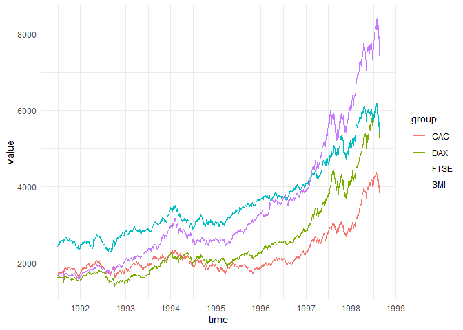
For the next examples we use flights departing from New York City in 2013.
library(nycflights13)
library(lubridate)
flights <- flights |>
mutate(date = as_date(time_hour))time_byflights_monthly <- flights |>
select(date, arr_delay) |>
time_by(date, "month")
flights_monthly
#> # A tibble: 336,776 x 2
#> # Time: date [12]
#> # Width: month
#> # Range: 2013-01-01 -- 2014-01-01
#> date arr_delay
#> <tm_ntrvl> <dbl>
#> 1 [2013-01-01, +1M) 11
#> 2 [2013-01-01, +1M) 20
#> 3 [2013-01-01, +1M) 33
#> 4 [2013-01-01, +1M) -18
#> 5 [2013-01-01, +1M) -25
#> 6 [2013-01-01, +1M) 12
#> 7 [2013-01-01, +1M) 19
#> 8 [2013-01-01, +1M) -14
#> 9 [2013-01-01, +1M) -8
#> 10 [2013-01-01, +1M) 8
#> # ℹ 336,766 more rowsWe can then use this to create a monthly summary of the number of flights and average arrival delay
flights_monthly |>
  f_summarise(n = n(),
            mean_arr_delay = mean(arr_delay, na.rm = TRUE))
#> # A tibble: 12 × 3
#>    date                  n mean_arr_delay
#>    <tm_ntrvl>        <int>          <dbl>
#>  1 [2013-01-01, +1M) 27004          6.13
#>  2 [2013-02-01, +1M) 24951          5.61
#>  3 [2013-03-01, +1M) 28834          5.81
#>  4 [2013-04-01, +1M) 28330         11.2
#>  5 [2013-05-01, +1M) 28796          3.52
#>  6 [2013-06-01, +1M) 28243         16.5
#>  7 [2013-07-01, +1M) 29425         16.7
#>  8 [2013-08-01, +1M) 29327          6.04
#>  9 [2013-09-01, +1M) 27574         -4.02
#> 10 [2013-10-01, +1M) 28889         -0.167
#> 11 [2013-11-01, +1M) 27268          0.461
#> 12 [2013-12-01, +1M) 28135         14.9
If the time unit is left unspecified, the time functions
try to find the highest time unit possible.
flights |>
  time_by(time_hour)
#> # A tibble: 336,776 x 20
#> # Time:     time_hour [6,936]
#> # Width:    hour
#> # Range:    2013-01-01 05:00:00 -- 2014-01-01
#>     year month   day dep_time sched_dep_time dep_delay arr_time sched_arr_time
#>    <int> <int> <int>    <int>          <int>     <dbl>    <int>          <int>
#>  1  2013     1     1      517            515         2      830            819
#>  2  2013     1     1      533            529         4      850            830
#>  3  2013     1     1      542            540         2      923            850
#>  4  2013     1     1      544            545        -1     1004           1022
#>  5  2013     1     1      554            600        -6      812            837
#>  6  2013     1     1      554            558        -4      740            728
#>  7  2013     1     1      555            600        -5      913            854
#>  8  2013     1     1      557            600        -3      709            723
#>  9  2013     1     1      557            600        -3      838            846
#> 10  2013     1     1      558            600        -2      753            745
#> # ℹ 336,766 more rows
#> # ℹ 12 more variables: arr_delay <dbl>, carrier <chr>, flight <int>,
#> #   tailnum <chr>, origin <chr>, dest <chr>, air_time <dbl>, distance <dbl>,
#> # hour <dbl>, minute <dbl>, time_hour <tm_ntrvl>, date <date>missing_dates(flights$date) # No missing dates
#> Date of length 0time_num_gaps(flights$time_hour) # Missing hours
#> [1] 1819To check for regularity use time_is_regular
hours <- sort(flights$time_hour)
time_is_regular(hours, "hours")
#> [1] FALSE
time_is_regular(hours, "hours", allow_gaps = TRUE, allow_dups = TRUE)
#> [1] TRUE

# By-group
time_num_gaps(flights$time_hour, g = flights$origin)
#>  EWR  JFK  LGA
#> 2489 1820 2468
time_is_regular(flights$time_hour, g = flights$origin)
#>   EWR   JFK   LGA
#> FALSE FALSE FALSEeu_stock <- eu_stock |>
mutate(date = date_decimal(time))
eu_stock |>
mutate(month_mean = time_roll_mean(value, window = months(3),
time = date,
g = group)) |>
time_ggplot(date, month_mean, group)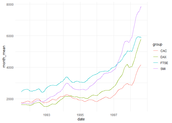
# Prerequisite: Create Time series with missing values
x <- ts(c(NA, 3, 4, NA, 6, NA, NA, 8))
g <- cheapr::seq_id(c(3, 5)) # Two groups of size 3 + 5

roll_na_fill(x) # Simple locf fill
#> Time Series:
#> Start = 1
#> End = 8
#> Frequency = 1
#> [1] NA  3  4  4  6  6  6  8
roll_na_fill(x, fill_limit = 1) # Fill up to 1 NA
#> Time Series:
#> Start = 1
#> End = 8
#> Frequency = 1
#> [1] NA  3  4  4  6  6 NA  8

roll_na_fill(x, g = g) # Very efficient on large data too
#> Time Series:
#> Start = 1
#> End = 8
#> Frequency = 1
#> [1] NA  3  4 NA  6  6  6  8
year_month and
year_quartertimeplyr has its own lightweight ‘yearmonth’ and `yearquarter’ classes inspired by the excellent ‘zoo’ and ‘tsibble’ packages.
today <- today()
year_month(today)
#> [1] "2025 Feb"
The underlying data for a year_month is the number of
months since 1 January 1970 (epoch).
unclass(year_month("1970-01-01"))
#> [1] 0
unclass(year_month("1971-01-01"))
#> [1] 12
To create a sequence of ‘year_months’, one can use base arithmetic
year_month(today) + 0:12
#>  [1] "2025 Feb" "2025 Mar" "2025 Apr" "2025 May" "2025 Jun" "2025 Jul"
#>  [7] "2025 Aug" "2025 Sep" "2025 Oct" "2025 Nov" "2025 Dec" "2026 Jan"
#> [13] "2026 Feb"
year_quarter(today) + 0:4
#> [1] "2025 Q1" "2025 Q2" "2025 Q3" "2025 Q4" "2026 Q1"time_elapsed()Let’s look at the time between consecutive flights for a specific flight number
set.seed(42)
flight_201 <- flights |>
  f_distinct(time_hour, flight) |>
  f_filter(flight %in% sample(flight, size = 1)) |>
  f_arrange(time_hour)

tail(sort(table(time_elapsed(flight_201$time_hour, "hours"))))
#>
#>  23  25  48   6  18  24
#>   2   3   4  33  34 218
Flight 201 seems to depart mostly consistently every 24 hours
We can efficiently do the same for all flight numbers
# We use fdistinct with sort as it's much faster and simpler to write
all_flights <- flights |>
  f_distinct(flight, time_hour, .sort = TRUE)
all_flights <- all_flights |>
  mutate(elapsed = time_elapsed(time_hour, g = flight, fill = 0))

# Flight numbers with largest relative deviation in time between flights
all_flights |>
  tidy_quantiles(elapsed, .by = flight, pivot = "wide") |>
  mutate(relative_iqr = p75 / p25) |>
  f_arrange(desc(relative_iqr))
#> # A tibble: 3,844 × 7
#>    flight    p0   p25   p50   p75  p100 relative_iqr
#>     <int> <dbl> <dbl> <dbl> <dbl> <dbl>        <dbl>
#>  1   3664     0    12    24 3252   6480         271
#>  2   5709     0    12    24 3080.  6137         257.
#>  3    513     0    12    24 2250.  4477         188.
#>  4   3364     0    12    24 2204.  4385         184.
#>  5   1578     0    24    48 4182.  8317         174.
#>  6   1830     0     1   167  168    168         168
#>  7   1569     0    18   105 2705   2787         150.
#>  8   1997     0    18    96 2158   8128         120.
#>  9    663     0    24   119 2604   3433         108.
#> 10    233     0     7    14  718   1422         103.
#> # ℹ 3,834 more rows
time_seq_id() allows us to create unique IDs for regular
sequences A new ID is created every time there is a gap in the
sequence
flights |>
  f_select(time_hour) |>
  f_arrange(time_hour) |>
  mutate(time_id = time_seq_id(time_hour)) |>
  f_filter(time_id != lag(time_id)) |>
  f_count(hour(time_hour))
#> # A tibble: 2 × 2
#>   `hour(time_hour)`     n
#>               <int> <int>
#> 1                 1     1
#> 2                 5   364
We can see that the gaps typically occur at 11pm and the sequence resumes at 5am.
calendar()flights_calendar <- flights |>
f_select(time_hour) |>
reframe(calendar(time_hour))Now that gaps in time have been filled and we have joined our date table, it is easy to count by any time dimension we like
flights_calendar |>
  f_count(isoyear, isoweek)
#> # A tibble: 53 × 3
#>    isoyear isoweek     n
#>      <int>   <int> <int>
#>  1    2013       1  5166
#>  2    2013       2  6114
#>  3    2013       3  6034
#>  4    2013       4  6049
#>  5    2013       5  6063
#>  6    2013       6  6104
#>  7    2013       7  6236
#>  8    2013       8  6381
#>  9    2013       9  6444
#> 10    2013      10  6546
#> # ℹ 43 more rows
flights_calendar |>
  f_count(isoweek = iso_week(time))
#> # A tibble: 53 × 2
#>    isoweek      n
#>    <chr>    <int>
#>  1 2013-W01  5166
#>  2 2013-W02  6114
#>  3 2013-W03  6034
#>  4 2013-W04  6049
#>  5 2013-W05  6063
#>  6 2013-W06  6104
#>  7 2013-W07  6236
#>  8 2013-W08  6381
#>  9 2013-W09  6444
#> 10 2013-W10  6546
#> # ℹ 43 more rows
flights_calendar |>
  f_count(month_l)
#> # A tibble: 12 × 2
#>    month_l     n
#>    <ord>   <int>
#>  1 Jan     27004
#>  2 Feb     24951
#>  3 Mar     28834
#>  4 Apr     28330
#>  5 May     28796
#>  6 Jun     28243
#>  7 Jul     29425
#>  8 Aug     29327
#>  9 Sep     27574
#> 10 Oct     28889
#> 11 Nov     27268
#> 12 Dec 28135time_seq()A lubridate version of seq() for dates and datetimes
start <- dmy(31012020)
end <- start + years(1)
seq(start, end, by = "month") # Base R version
#>  [1] "2020-01-31" "2020-03-02" "2020-03-31" "2020-05-01" "2020-05-31"
#>  [6] "2020-07-01" "2020-07-31" "2020-08-31" "2020-10-01" "2020-10-31"
#> [11] "2020-12-01" "2020-12-31" "2021-01-31"
time_seq(start, end, "month") # lubridate version
#>  [1] "2020-01-31" "2020-03-01" "2020-03-31" "2020-05-01" "2020-05-31"
#>  [6] "2020-07-01" "2020-07-31" "2020-08-31" "2020-10-01" "2020-10-31"
#> [11] "2020-12-01" "2020-12-31" "2021-01-31"
time_seq() doesn’t mind mixing dates and datetimes
time_seq(start, as_datetime(end), "2 weeks")
#>  [1] "2020-01-31 UTC" "2020-02-14 UTC" "2020-02-28 UTC" "2020-03-13 UTC"
#>  [5] "2020-03-27 UTC" "2020-04-10 UTC" "2020-04-24 UTC" "2020-05-08 UTC"
#>  [9] "2020-05-22 UTC" "2020-06-05 UTC" "2020-06-19 UTC" "2020-07-03 UTC"
#> [13] "2020-07-17 UTC" "2020-07-31 UTC" "2020-08-14 UTC" "2020-08-28 UTC"
#> [17] "2020-09-11 UTC" "2020-09-25 UTC" "2020-10-09 UTC" "2020-10-23 UTC"
#> [21] "2020-11-06 UTC" "2020-11-20 UTC" "2020-12-04 UTC" "2020-12-18 UTC"
#> [25] "2021-01-01 UTC" "2021-01-15 UTC" "2021-01-29 UTC"
It is also vectorised
# 3 sequences
time_seq(from = start,
         to = end,
         timespan("months", 1:3))
#>  [1] "2020-01-31" "2020-03-01" "2020-03-31" "2020-05-01" "2020-05-31"
#>  [6] "2020-07-01" "2020-07-31" "2020-08-31" "2020-10-01" "2020-10-31"
#> [11] "2020-12-01" "2020-12-31" "2021-01-31" "2020-01-31" "2020-03-31"
#> [16] "2020-05-31" "2020-07-31" "2020-10-01" "2020-12-01" "2021-01-31"
#> [21] "2020-01-31" "2020-05-01" "2020-07-31" "2020-10-31" "2021-01-31"
# Equivalent to
c(time_seq(start, end, "month"),
  time_seq(start, end, "2 months"),
  time_seq(start, end, "3 months"))
#>  [1] "2020-01-31" "2020-03-01" "2020-03-31" "2020-05-01" "2020-05-31"
#>  [6] "2020-07-01" "2020-07-31" "2020-08-31" "2020-10-01" "2020-10-31"
#> [11] "2020-12-01" "2020-12-31" "2021-01-31" "2020-01-31" "2020-03-31"
#> [16] "2020-05-31" "2020-07-31" "2020-10-01" "2020-12-01" "2021-01-31"
#> [21] "2020-01-31" "2020-05-01" "2020-07-31" "2020-10-31" "2021-01-31"time_seq_sizes()Vectorised function that calculates time sequence lengths
seq_lengths <- time_seq_sizes(start, start + days(c(1, 10, 20)),
                              timespan("days", c(1, 5, 10)))
seq_lengths
#> [1] 2 3 3

# Use time_seq_v2() if you know the sequence lengths
seqs <- time_seq_v2(seq_lengths, start, timespan("days", c(1, 5, 10)))
seqs
#> [1] "2020-01-31" "2020-02-01" "2020-01-31" "2020-02-05" "2020-02-10"
#> [6] "2020-01-31" "2020-02-10" "2020-02-20"iso_week()Simple function to get formatted ISO weeks.
iso_week(today())
#> [1] "2025-W09"
iso_week(today(), day = TRUE)
#> [1] "2025-W09-5"
iso_week(today(), year = FALSE)
#> [1] "W09"time_cut()Create pretty time axes using time_breaks()
times <- flights$time_hour
dates <- flights$date

date_breaks <- time_breaks(dates, n = 12)
time_breaks <- time_breaks(times, n = 12, time_floor = TRUE)

weekly_data <- flights |>
    time_by(date, "week",
            .name = "date") |>
    f_count()
weekly_data |>
  ggplot(aes(x = interval_start(date), y = n)) +
  geom_bar(stat = "identity", fill = "#0072B2") +
scale_x_date(breaks = date_breaks, labels = scales::label_date_short()) 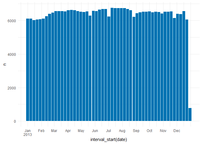
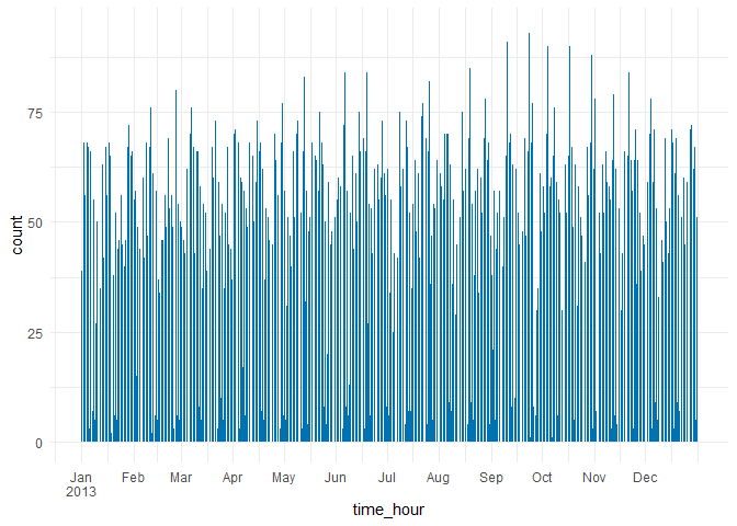
flights |>
  ggplot(aes(x = time_hour)) +
  geom_bar(fill = "#0072B2") +
  scale_x_datetime(breaks = time_breaks, labels = scales::label_date_short())