![]()
![]()
![]()
You can install the sparklyr package from CRAN as follows:
install.packages("sparklyr")You should also install a local version of Spark for development purposes:
library(sparklyr)
spark_install()
To upgrade to the latest version of sparklyr, run the following command and restart your r session:
install.packages("devtools")
devtools::install_github("sparklyr/sparklyr")You can connect to both local instances of Spark as well as remote Spark clusters. Here we’ll connect to a local instance of Spark via the spark_connect function:
library(sparklyr)
sc <- spark_connect(master = "local")
The returned Spark connection (sc) provides a remote
dplyr data source to the Spark cluster.
For more information on connecting to remote Spark clusters see the Deployment section of the sparklyr website.
We can now use all of the available dplyr verbs against the tables within the cluster.
We’ll start by copying some datasets from R into the Spark cluster (note that you may need to install the nycflights13 and Lahman packages in order to execute this code):
install.packages(c("nycflights13", "Lahman"))library(dplyr)
iris_tbl <- copy_to(sc, iris, overwrite = TRUE)
flights_tbl <- copy_to(sc, nycflights13::flights, "flights", overwrite = TRUE)
batting_tbl <- copy_to(sc, Lahman::Batting, "batting", overwrite = TRUE)
src_tbls(sc)
#> [1] "batting" "flights" "iris"To start with here’s a simple filtering example:
# filter by departure delay and print the first few records
flights_tbl %>% filter(dep_delay == 2)
#> # Source:   SQL [?? x 19]
#> # Database: spark_connection
#>     year month   day dep_time sched_dep_time dep_delay
#>    <int> <int> <int>    <int>          <int>     <dbl>
#>  1  2013     1     1      517            515         2
#>  2  2013     1     1      542            540         2
#>  3  2013     1     1      702            700         2
#>  4  2013     1     1      715            713         2
#>  5  2013     1     1      752            750         2
#>  6  2013     1     1      917            915         2
#>  7  2013     1     1      932            930         2
#>  8  2013     1     1     1028           1026         2
#>  9  2013     1     1     1042           1040         2
#> 10  2013     1     1     1231           1229         2
#> # ℹ more rows
#> # ℹ 13 more variables: arr_time <int>,
#> #   sched_arr_time <int>, arr_delay <dbl>, carrier <chr>,
#> #   flight <int>, tailnum <chr>, origin <chr>, dest <chr>,
#> #   air_time <dbl>, distance <dbl>, hour <dbl>,
#> #   minute <dbl>, time_hour <dttm>
Introduction to
dplyr provides additional dplyr examples you can try.
For example, consider the last example from the tutorial which plots
data on flight delays:
delay <- flights_tbl %>%
  group_by(tailnum) %>%
  summarise(count = n(), dist = mean(distance), delay = mean(arr_delay)) %>%
  filter(count > 20, dist < 2000, !is.na(delay)) %>%
  collect()

# plot delays
library(ggplot2)
ggplot(delay, aes(dist, delay)) +
  geom_point(aes(size = count), alpha = 1/2) +
  geom_smooth() +
  scale_size_area(max_size = 2)
#> `geom_smooth()` using method = 'gam' and formula = 'y ~
#> s(x, bs = "cs")'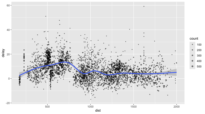
dplyr window functions are also supported, for example:
batting_tbl %>%
  select(playerID, yearID, teamID, G, AB:H) %>%
  arrange(playerID, yearID, teamID) %>%
  group_by(playerID) %>%
  filter(min_rank(desc(H)) <= 2 & H > 0)
#> # Source:     SQL [?? x 7]
#> # Database:   spark_connection
#> # Groups:     playerID
#> # Ordered by: playerID, yearID, teamID
#>    playerID  yearID teamID     G    AB     R     H
#>    <chr>      <int> <chr>  <int> <int> <int> <int>
#>  1 abadijo01   1875 PH3       11    45     3    10
#>  2 abadijo01   1875 BR2        1     4     1     1
#>  3 abbeybe01   1896 BRO       25    63     7    12
#>  4 abbeybe01   1892 WAS       27    75     5     9
#>  5 abbeych01   1894 WAS      129   523    95   164
#>  6 abbeych01   1895 WAS      133   516   102   142
#>  7 abbotfr01   1903 CLE       77   255    25    60
#>  8 abbotfr01   1905 PHI       42   128     9    25
#>  9 abbotky01   1992 PHI       31    29     1     2
#> 10 abbotky01   1995 PHI       18     2     1     1
#> # ℹ more rows
For additional documentation on using dplyr with Spark see the dplyr section of the sparklyr website.
It’s also possible to execute SQL queries directly against tables
within a Spark cluster. The spark_connection object
implements a DBI interface
for Spark, so you can use dbGetQuery() to execute SQL and
return the result as an R data frame:
library(DBI)
iris_preview <- dbGetQuery(sc, "SELECT * FROM iris LIMIT 10")
iris_preview
#>    Sepal_Length Sepal_Width Petal_Length Petal_Width
#> 1           5.1         3.5          1.4         0.2
#> 2           4.9         3.0          1.4         0.2
#> 3           4.7         3.2          1.3         0.2
#> 4           4.6         3.1          1.5         0.2
#> 5           5.0         3.6          1.4         0.2
#> 6           5.4         3.9          1.7         0.4
#> 7           4.6         3.4          1.4         0.3
#> 8           5.0         3.4          1.5         0.2
#> 9           4.4         2.9          1.4         0.2
#> 10          4.9         3.1          1.5         0.1
#>    Species
#> 1   setosa
#> 2   setosa
#> 3   setosa
#> 4   setosa
#> 5   setosa
#> 6   setosa
#> 7   setosa
#> 8   setosa
#> 9   setosa
#> 10 setosaYou can orchestrate machine learning algorithms in a Spark cluster via the machine learning functions within sparklyr. These functions connect to a set of high-level APIs built on top of DataFrames that help you create and tune machine learning workflows.
Here’s an example where we use ml_linear_regression
to fit a linear regression model. We’ll use the built-in
mtcars dataset, and see if we can predict a car’s fuel
consumption (mpg) based on its weight (wt),
and the number of cylinders the engine contains (cyl).
We’ll assume in each case that the relationship between mpg
and each of our features is linear.
# copy mtcars into spark
mtcars_tbl <- copy_to(sc, mtcars, overwrite = TRUE)

# transform our data set, and then partition into 'training', 'test'
partitions <- mtcars_tbl %>%
  filter(hp >= 100) %>%
  mutate(cyl8 = cyl == 8) %>%
  sdf_partition(training = 0.5, test = 0.5, seed = 1099)

# fit a linear model to the training dataset
fit <- partitions$training %>%
  ml_linear_regression(response = "mpg", features = c("wt", "cyl"))
fit
#> Formula: mpg ~ wt + cyl
#>
#> Coefficients:
#> (Intercept)          wt         cyl
#>  37.1464554  -4.3408005  -0.5830515
For linear regression models produced by Spark, we can use
summary() to learn a bit more about the quality of our fit,
and the statistical significance of each of our predictors.
summary(fit)
#> Deviance Residuals:
#>     Min      1Q  Median      3Q     Max
#> -2.5134 -0.9158 -0.1683  1.1503  2.1534
#>
#> Coefficients:
#> (Intercept)          wt         cyl
#>  37.1464554  -4.3408005  -0.5830515
#>
#> R-Squared: 0.9428
#> Root Mean Squared Error: 1.409
Spark machine learning supports a wide array of algorithms and feature transformations and as illustrated above it’s easy to chain these functions together with dplyr pipelines. To learn more see the machine learning section.
You can read and write data in CSV, JSON, and Parquet formats. Data can be stored in HDFS, S3, or on the local filesystem of cluster nodes.
temp_csv <- tempfile(fileext = ".csv")
temp_parquet <- tempfile(fileext = ".parquet")
temp_json <- tempfile(fileext = ".json")

spark_write_csv(iris_tbl, temp_csv)
iris_csv_tbl <- spark_read_csv(sc, "iris_csv", temp_csv)

spark_write_parquet(iris_tbl, temp_parquet)
iris_parquet_tbl <- spark_read_parquet(sc, "iris_parquet", temp_parquet)

spark_write_json(iris_tbl, temp_json)
iris_json_tbl <- spark_read_json(sc, "iris_json", temp_json)

src_tbls(sc)
#> [1] "batting"      "flights"      "iris"
#> [4] "iris_csv"     "iris_json"    "iris_parquet"
#> [7] "mtcars"You can execute arbitrary r code across your cluster using
spark_apply(). For example, we can apply
rgamma over iris as follows:
spark_apply(iris_tbl, function(data) {
  data[1:4] + rgamma(1,2)
})
#> # Source:   table<`sparklyr_tmp__752f1c17_51c6_45bc_a22e_fa06e1ebac58`> [?? x 4]
#> # Database: spark_connection
#>    Sepal_Length Sepal_Width Petal_Length Petal_Width
#>           <dbl>       <dbl>        <dbl>       <dbl>
#>  1        10.1         8.48         6.38        5.18
#>  2         9.88        7.98         6.38        5.18
#>  3         9.68        8.18         6.28        5.18
#>  4         9.58        8.08         6.48        5.18
#>  5         9.98        8.58         6.38        5.18
#>  6        10.4         8.88         6.68        5.38
#>  7         9.58        8.38         6.38        5.28
#>  8         9.98        8.38         6.48        5.18
#>  9         9.38        7.88         6.38        5.18
#> 10         9.88        8.08         6.48        5.08
#> # ℹ more rows
You can also group by columns to perform an operation over each group of rows and make use of any package within the closure:
spark_apply(
  iris_tbl,
  function(e) broom::tidy(lm(Petal_Width ~ Petal_Length, e)),
  columns = c("term", "estimate", "std.error", "statistic", "p.value"),
  group_by = "Species"
)
#> # Source:   table<`sparklyr_tmp__11d902f5_6218_41db_85dd_72c5ebe98eab`> [?? x 6]
#> # Database: spark_connection
#>   Species    term      estimate std.error statistic  p.value
#>   <chr>      <chr>        <dbl>     <dbl>     <dbl>    <dbl>
#> 1 versicolor (Interce…  -0.0843    0.161     -0.525 6.02e- 1
#> 2 versicolor Petal_Le…   0.331     0.0375     8.83  1.27e-11
#> 3 virginica  (Interce…   1.14      0.379      2.99  4.34e- 3
#> 4 virginica  Petal_Le…   0.160     0.0680     2.36  2.25e- 2
#> 5 setosa     (Interce…  -0.0482    0.122     -0.396 6.94e- 1
#> 6 setosa Petal_Le… 0.201 0.0826 2.44 1.86e- 2The facilities used internally by sparklyr for its dplyr
and machine learning interfaces are available to extension packages.
Since Spark is a general purpose cluster computing system there are many
potential applications for extensions (e.g. interfaces to custom
machine learning pipelines, interfaces to 3rd party Spark packages,
etc.).
Here’s a simple example that wraps a Spark text file line counting function with an R function:
# write a CSV
tempfile <- tempfile(fileext = ".csv")
write.csv(nycflights13::flights, tempfile, row.names = FALSE, na = "")

# define an R interface to Spark line counting
count_lines <- function(sc, path) {
  spark_context(sc) %>%
    invoke("textFile", path, 1L) %>%
      invoke("count")
}

# call spark to count the lines of the CSV
count_lines(sc, tempfile)
#> [1] 336777
To learn more about creating extensions see the Extensions section of the sparklyr website.
You can cache a table into memory with:
tbl_cache(sc, "batting")and unload from memory using:
tbl_uncache(sc, "batting")You can view the Spark web console using the spark_web()
function:
spark_web(sc)You can show the log using the spark_log() function:
spark_log(sc, n = 10)
#> {"ts":"2025-03-18T05:33:03.487Z","level":"INFO","msg":"Running task 0.0 in stage 90.0 (TID 127)","context":{"task_name":"task 0.0 in stage 90.0 (TID 127)"},"logger":"Executor"}
#> {"ts":"2025-03-18T05:33:03.491Z","level":"INFO","msg":"Task (TID 127) input split: file:/var/folders/y_/f_0cx_291nl0s8h26t4jg6ch0000gp/T/RtmpTDeQSI/fileaff16a4bc7cf.csv:0+33313106","context":{"input_split":"file:/var/folders/y_/f_0cx_291nl0s8h26t4jg6ch0000gp/T/RtmpTDeQSI/fileaff16a4bc7cf.csv:0+33313106","task_id":"127","task_name":"task 0.0 in stage 90.0 (TID 127)"},"logger":"HadoopRDD"}
#> {"ts":"2025-03-18T05:33:03.597Z","level":"INFO","msg":"Finished task 0.0 in stage 90.0 (TID 127). 1078 bytes result sent to driver","context":{"num_bytes":"1078","task_name":"task 0.0 in stage 90.0 (TID 127)"},"logger":"Executor"}
#> {"ts":"2025-03-18T05:33:03.598Z","level":"INFO","msg":"Finished task 0.0 in stage 90.0 (TID 127) in 116 ms on localhost (executor driver) (1/1)","context":{"duration":"116","executor_id":"driver","host":"localhost","num_successful_tasks":"1","num_tasks":"1","task_name":"task 0.0 in stage 90.0 (TID 127)"},"logger":"TaskSetManager"}
#> {"ts":"2025-03-18T05:33:03.598Z","level":"INFO","msg":"Removed TaskSet 90.0 whose tasks have all completed, from pool ","context":{"pool_name":"","stage_attempt":"0","stage_id":"90"},"logger":"TaskSchedulerImpl"}
#> {"ts":"2025-03-18T05:33:03.598Z","level":"INFO","msg":"ResultStage 90 (count at NativeMethodAccessorImpl.java:0) finished in 118 ms","context":{"stage":"ResultStage 90","stage_name":"count at NativeMethodAccessorImpl.java:0","time_units":"118"},"logger":"DAGScheduler"}
#> {"ts":"2025-03-18T05:33:03.598Z","level":"INFO","msg":"Job 74 is finished. Cancelling potential speculative or zombie tasks for this job","context":{"job_id":"74"},"logger":"DAGScheduler"}
#> {"ts":"2025-03-18T05:33:03.598Z","level":"INFO","msg":"Canceling stage 90","context":{"stage_id":"90"},"logger":"TaskSchedulerImpl"}
#> {"ts":"2025-03-18T05:33:03.598Z","level":"INFO","msg":"Killing all running tasks in stage 90: Stage finished","context":{"reason":"Stage finished","stage_id":"90"},"logger":"TaskSchedulerImpl"}
#> {"ts":"2025-03-18T05:33:03.598Z","level":"INFO","msg":"Job 74 finished: count at NativeMethodAccessorImpl.java:0, took 118.374959 ms","context":{"call_site_short_form":"count at NativeMethodAccessorImpl.java:0","job_id":"74","time":"118.374959"},"logger":"DAGScheduler"}
Finally, we disconnect from Spark:
spark_disconnect(sc)The RStudio IDE includes integrated support for Spark and the sparklyr package, including tools for:
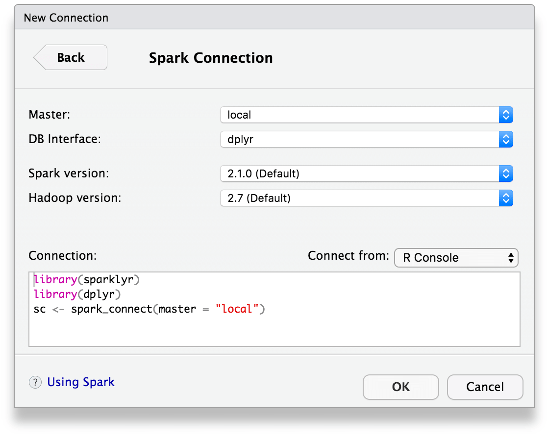
Once you’ve installed the sparklyr package, you should find a new Spark pane within the IDE. This pane includes a New Connection dialog which can be used to make connections to local or remote Spark instances:
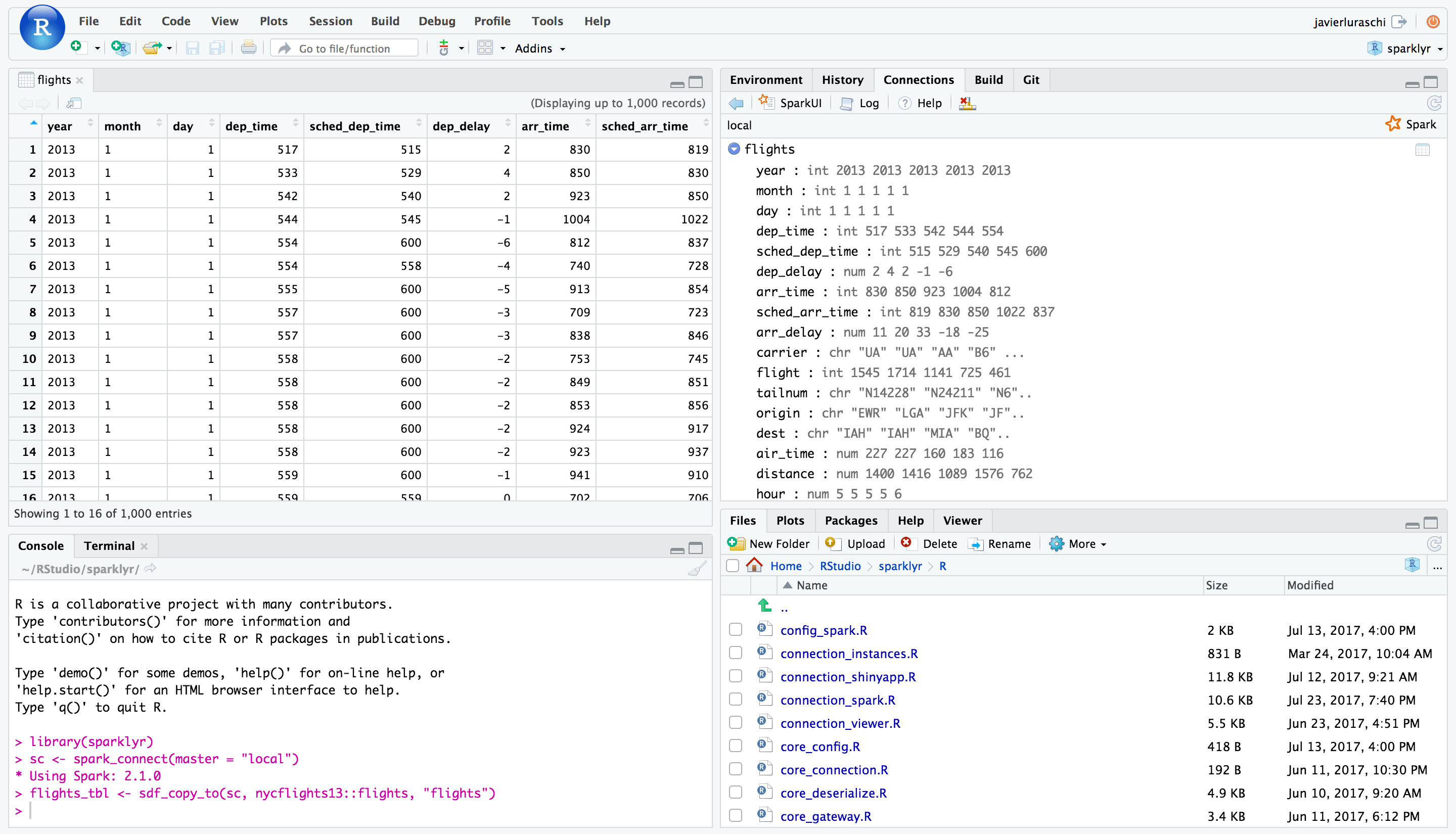
Once you’ve connected to Spark you’ll be able to browse the tables contained within the Spark cluster and preview Spark DataFrames using the standard RStudio data viewer:
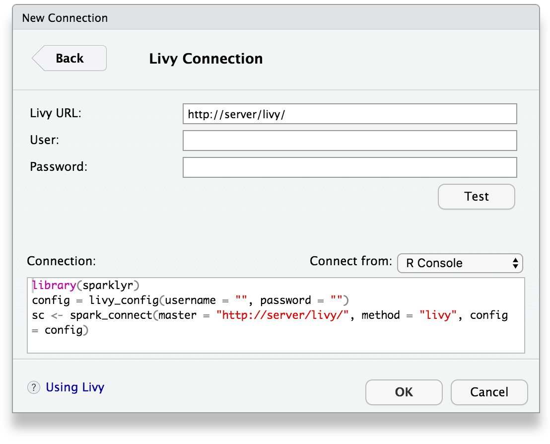
You can also connect to Spark through Livy through a new connection dialog:
rsparkling is a CRAN package from H2O that extends sparklyr to provide an interface into Sparkling Water. For instance, the following example installs, configures and runs h2o.glm:
library(rsparkling)
library(sparklyr)
library(dplyr)
library(h2o)

sc <- spark_connect(master = "local", version = "2.3.2")
mtcars_tbl <- copy_to(sc, mtcars, "mtcars", overwrite = TRUE)

mtcars_h2o <- as_h2o_frame(sc, mtcars_tbl, strict_version_check = FALSE)

mtcars_glm <- h2o.glm(x = c("wt", "cyl"),
                      y = "mpg",
                      training_frame = mtcars_h2o,
lambda_search = TRUE)mtcars_glm#> Model Details:
#> ==============
#>
#> H2ORegressionModel: glm
#> Model ID: GLM_model_R_1527265202599_1
#> GLM Model: summary
#> family link regularization
#> 1 gaussian identity Elastic Net (alpha = 0.5, lambda = 0.1013 )
#> lambda_search
#> 1 nlambda = 100, lambda.max = 10.132, lambda.min = 0.1013, lambda.1se = -1.0
#> number_of_predictors_total number_of_active_predictors
#> 1 2 2
#> number_of_iterations training_frame
#> 1 100 frame_rdd_31_ad5c4e88ec97eb8ccedae9475ad34e02
#>
#> Coefficients: glm coefficients
#> names coefficients standardized_coefficients
#> 1 Intercept 38.941654 20.090625
#> 2 cyl -1.468783 -2.623132
#> 3 wt -3.034558 -2.969186
#>
#> H2ORegressionMetrics: glm
#> ** Reported on training data. **
#>
#> MSE: 6.017684
#> RMSE: 2.453097
#> MAE: 1.940985
#> RMSLE: 0.1114801
#> Mean Residual Deviance : 6.017684
#> R^2 : 0.8289895
#> Null Deviance :1126.047
#> Null D.o.F. :31
#> Residual Deviance :192.5659
#> Residual D.o.F. :29
#> AIC :156.2425spark_disconnect(sc)Livy enables remote connections to Apache Spark clusters. However, please notice that connecting to Spark clusters through Livy is much slower than any other connection method.
Before connecting to Livy, you will need the connection information
to an existing service running Livy. Otherwise, to test
livy in your local environment, you can install it and run
it locally as follows:
livy_install()livy_service_start()To connect, use the Livy service address as master and
method = "livy" in spark_connect(). Once
connection completes, use sparklyr as usual, for
instance:
sc <- spark_connect(master = "http://localhost:8998", method = "livy", version = "3.0.0")
copy_to(sc, iris, overwrite = TRUE)

spark_disconnect(sc)
Once you are done using livy locally, you should stop
this service with:
livy_service_stop()To connect to remote livy clusters that support basic
authentication connect as:
config <- livy_config(username="<username>", password="<password>")
sc <- spark_connect(master = "<address>", method = "livy", config = config)
spark_disconnect(sc)sparklyr is able to interact with Databricks
Connect v2 via a new extension called pysparklyr. To
learn how to use, and the latest updates on this integration see the
article in sparklyr’s official website.