The goal of simDNAmixtures is to provide an easy to use workflow for simulating single source or mixed forensic DNA profiles. These simulations are used in research and validation related to probabilistic genotyping systems and also in studies on relationship testing.
The simDNAmixtures package supports simulation of:
Autosomal STR profiles (e.g. GlobalFiler™)
Autosomal SNP profiles (e.g. Kintelligence or FORCE)
YSTR profiles (e.g. Yfiler™ Plus)
Genotypes of the sample contributors may be provided as inputs. For autosomal profiles (STRs or SNPs) it is also possible to sample genotypes according to allele frequencies and a pedigree.
To install simDNAmixtures from CRAN:
install.packages("simDNAmixtures")Alternatively, you can install the development version of simDNAmixtures from GitHub with:
# install.packages("devtools")
devtools::install_github("mkruijver/simDNAmixtures")This example demonstrates how a mixed STR profile comprising two siblings can be simulated. More comprehensive examples of how to set up a simulation study can be found in the vignettes.
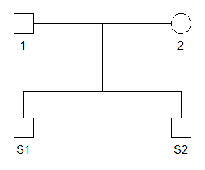
The first step is to define a pedigree with the two siblings and their parents using the pedtools package.
library(simDNAmixtures)
library(pedtools)

ped_fs <- nuclearPed(children = c("S1", "S2"))
plot(ped_fs)
Further, we load provided data including allele frequencies and data related to the GlobalFiler™ kit such as the locus names, size regression and stutter model.
# load allele frequencies
freqs <- read_allele_freqs(system.file("extdata","FBI_extended_Cauc_022024.csv",
                           package = "simDNAmixtures"))

# load kit data
gf <- gf_configuration()
We are now ready to sample a mixed STR profile. A gamma model is used with \(\mu\) sampled uniformly between 50 and 5000 rfu and a coefficient of variation between 5 and 35%.
set.seed(1)

sampling_parameters <- list(min_mu = 50., max_mu = 5e3,
                           min_cv = 0.05, max_cv = 0.35,
                           degradation_shape1 = 0, degradation_shape2 = 0)

mixtures <- sample_mixtures(n = 1, contributors = c("S1", "S2"),
                            pedigree = ped_fs, freqs = freqs,
                            sampling_parameters = sampling_parameters,
                            model_settings = gf$gamma_settings,
                            sample_model = sample_gamma_model)
The simulation results are stored in the mixtures
object. Note that the results_directory argument to the
sample_mixtures function may be used to automatically write
results to disk. Below we print the simulated mixture data stored as
mixtures$samples[[1]]$mixture.
| Locus | Allele | Height | Size |
|---|---|---|---|
| D3S1358 | 14 | 216 | 117.33 |
| D3S1358 | 15 | 4159 | 121.40 |
| vWA | 14 | 1512 | 168.84 |
| vWA | 17 | 180 | 180.95 |
| vWA | 18 | 2554 | 184.99 |
| vWA | 19 | 695 | 189.02 |
| D16S539 | 9 | 1315 | 243.61 |
| D16S539 | 10 | 1003 | 247.64 |
| D16S539 | 12 | 138 | 255.70 |
| D16S539 | 13 | 1990 | 259.73 |
| CSF1PO | 10 | 635 | 298.34 |
| CSF1PO | 11 | 1195 | 302.30 |
| CSF1PO | 12 | 1879 | 306.26 |
| TPOX | 8 | 847 | 349.70 |
| TPOX | 9 | 1185 | 353.72 |
| TPOX | 11 | 102 | 361.78 |
| TPOX | 12 | 1616 | 365.81 |
| AMEL | X | 1549 | 98.50 |
| AMEL | Y | 2616 | 104.50 |
| D8S1179 | 10 | 1571 | 134.96 |
| D8S1179 | 13 | 995 | 147.26 |
| D8S1179 | 14 | 702 | 151.36 |
| D21S11 | 29 | 267 | 203.65 |
| D21S11 | 30 | 1952 | 207.69 |
| D21S11 | 30.2 | 254 | 208.50 |
| D21S11 | 31.2 | 1910 | 212.54 |
| D18S51 | 12 | 374 | 281.63 |
| D18S51 | 13 | 2473 | 285.67 |
| D18S51 | 14 | 1789 | 289.71 |
| D2S441 | 9 | 83 | 81.31 |
| D2S441 | 10 | 3538 | 85.37 |
| D2S441 | 11 | 851 | 89.42 |
| D19S433 | 13 | 145 | 145.75 |
| D19S433 | 13.2 | 971 | 146.55 |
| D19S433 | 14 | 2355 | 149.74 |
| TH01 | 8 | 2821 | 195.22 |
| TH01 | 9 | 2190 | 199.38 |
| FGA | 21 | 97 | 255.94 |
| FGA | 22 | 1328 | 260.01 |
| FGA | 23 | 1614 | 264.08 |
| FGA | 24 | 73 | 268.15 |
| D22S1045 | 11 | 2201 | 97.51 |
| D22S1045 | 14 | 126 | 106.47 |
| D22S1045 | 15 | 1513 | 109.46 |
| D5S818 | 10 | 324 | 150.82 |
| D5S818 | 11 | 1955 | 154.87 |
| D5S818 | 12 | 995 | 158.92 |
| D5S818 | 13 | 1777 | 162.97 |
| D13S317 | 11 | 184 | 222.97 |
| D13S317 | 12 | 4363 | 227.02 |
| D7S820 | 11 | 2551 | 282.34 |
| D7S820 | 12 | 660 | 286.32 |
| SE33 | 17 | 1425 | 358.71 |
| SE33 | 18 | 903 | 362.77 |
| SE33 | 19 | 225 | 366.84 |
| SE33 | 29.2 | 269 | 408.32 |
| SE33 | 30.2 | 2077 | 412.39 |
| D10S1248 | 13 | 1831 | 105.53 |
| D10S1248 | 14 | 656 | 109.53 |
| D1S1656 | 12 | 873 | 172.23 |
| D1S1656 | 13 | 773 | 176.45 |
| D1S1656 | 16 | 714 | 189.10 |
| D1S1656 | 17.3 | 630 | 194.58 |
| D12S391 | 17 | 132 | 228.10 |
| D12S391 | 18 | 902 | 232.07 |
| D12S391 | 19 | 124 | 236.04 |
| D12S391 | 20 | 1475 | 240.01 |
| D12S391 | 22 | 1053 | 247.96 |
| D2S1338 | 17 | 672 | 304.78 |
| D2S1338 | 19 | 1505 | 312.82 |
| D2S1338 | 22 | 705 | 324.87 |
| D2S1338 | 24 | 894 | 332.91 |
The genotypes of the two contributors are available as
mixtures$samples[[1]]$contributor_genotypes.
|
|